Description
Clicking on any thumbnail image below will bring up the full-size
version of the same image. Both thumbnails and full-size images are
compressed and thus the displayed volume renderings will not match
pixel-to-pixel the output of your implementation.
Introduction
Your task is to write all code managing the octree data structure of a
volume rendering system. In addition to coding, you must analyze the
time and space complexity of the routines you write. We have written
all code handling geometrical and graphical computations for you; your
code is focused on octrees, which are a challenging extension of
binary trees.
Policies
General information and policies regarding the project are available
in detail, and we
strongly recommend you read them; to summarize:
- The project is designed to consume one person-week of analysis and
coding.
- The recommended development platform is Sun workstations. We will
grade your project on one of the Sweet Hall epic
workstations. Therefore, it's absolutely critical that your submitted
code compiles and runs on an epic.
- You may work in teams of no more than two students, and turn in a
single project per group. Honor code violations will be severely
punished.
After you read this document, another WWW page will help you get started, including guiding you
through account setup, using the demo executable, and compiling and
testing your code. If you have any questions, please contact the TAs
or the instructor. To help us help you efficiently, make sure that
Background and motivation
Before delving into the details of your task, some fundamental
background information on volumes and their rendering would be useful.
For our purposes, a volume is the three-dimensional analog of
a square image: it is a 3D array of bytes, whose length L is the same
along every dimension; also, this length is an exact, non-negative
power of 2. By analogy to images, where individual elements of the 2D
image array are called pixels, the elements of a volume are called
voxels.
Each pixel of a monochrome image has a value between 0 and 255,
representing a shade of gray from the darkest black to the brightest
white. To gain some intuition for voxel values, try to visualize an
object, such as a person's head, trapped inside a big cube,
corresponding to our volume; now subdivide this cube into tiny cells,
each corresponding to a voxel. Some cells will be empty (with
corresponding voxels having a zero value), while other cells will
contain physiological structures, such as tissue, bone, muscles, etc.;
the value of a non-empty voxel is proportional to the average material
density of the structures contained in the corresponding cell.
The above description fits exactly the kind of volume generated by a
Computerized Tomography (CT) scanner; and, a Magnetic Resonance
Imaging (MRI) device measures the local concentration of hydrogen
atoms. We can also use 3D computer models (VRML, etc.) to construct
volumes that represent the skin of an object, using a process called
scan conversion: a voxel's value is proportional to the skin
area enclosed by the associated cell; this is the kind of data we will
use.
Volume datasets are huge, with 80MB being fairly typical. This causes
two major headaches:
- Storage
- Storing a volume as a raw sequence of voxel values is wasteful:
in practice, most cells are empty; also, we frequently don't care
about small variations in value between adjacent voxels. So, we'd like
to come up with an alternative storage scheme that repeatedly
coalesces nearby similar cells into bigger and bigger cells, and then
only stores one value for each surviving cell. That's the purpose an
octree serves.
- Comprehension
- Turning raw bytes into useful information (i.e. into something
that a doctor can understand) is a hard task. The solution relies on
the fact that nothing matches the ability of our visual system when it
comes to interpreting huge amounts of data: it's much easier to detect
patterns in the contents of a big 2D array by drawing each value as a
screen pixel than printing byte values on the terminal. So we need a
process that, in general terms, will turn a volume into something we
can look at. That's what volume rendering is about.
Octrees
An octree is a tree with eight children for each internal node. And
that's about it as far as the data structure itself is concerned. What
makes octrees interesting is the way we interpret this data structure
in relation to volumes.
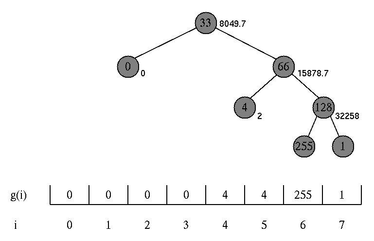
Let's start with binary trees and 1D functions. Imagine a scalar
function f(i) mapping each of the integers i between 0 and 7 to a
byte. Build a complete binary tree of depth 3, and label its leaves
with f(i) as shown below. Label the interior node n with the average
value of the leaves of n's subtree; also, write next to each interior
node the variance of (the values in) the same leaves. (NB: the average
and variance of the subtree leaves is not necessarily the
same as the average and variance of the two children of n; we never
use the latter quantities.)
Representing f using this tree is an overkill: none of the interior
node is really necessary. However, instead of throwing away the
interior nodes in order to represent f concisely, we'll proceed as
follows:
- First, we come up with a way to represent a function using an
incomplete tree: we imagine that any branch which is not grown to full
depth would have produced leaves with values identical to that of the
last existing node on the branch, if it were to be fully
grown. (Please read this again.)
- Next, we generate such a reduced tree by taking the original one
and discarding all subtrees rooted at a node with zero variance (but
we don't discard the root itself). In the above example, we are left
with the gray nodes only.
This process is called lossless compression: useless data is
thrown away without information loss. Now let's take this idea a step
further. Before, we pruned a subtree if the root variance was zero;
now, we'll prune a subtree if the variance of all (internal)
subtree nodes does not exceed a user-defined variance limit
T. Returning to our example, any T in the range [2,32258) produces the
tree shown below. The functional interpretation g(i) of the resulting
tree is an approximation to the original function f(i). This process
is called lossy compression.

Task 1 [5 points]: Lossless compression sounds like a
special case of lossy compression, with T being zero... except that
our lossless scheme looks only at the root before pruning, ignoring
all other subtree nodes. Show that, with T = 0, lossy compression is
identical to lossless compression.
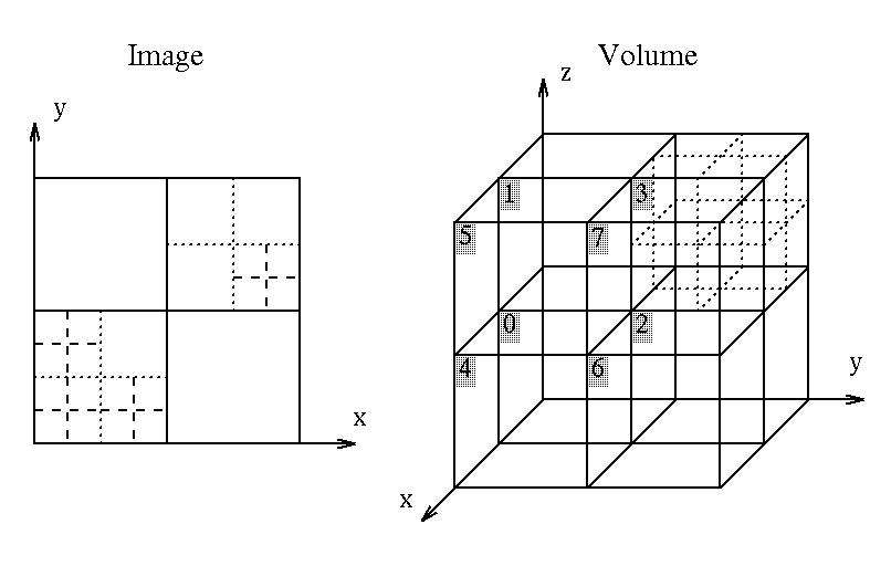
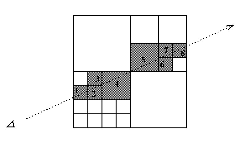
The same ideas as above can be applied in two and three dimensions. In
two dimensions, we use a quadtree to represent a scalar
function mapping each integer pair (x,y) - with x and y between 0 and
(L-1) - to a byte. An internal quadtree node has four children: one
for the top right subsquare, one for the top left, one for bottom
right, one for bottom left.
In three dimensions, we use an octree, where each internal
node has eight children, one for each subcell (subcube) of the parent
cell (cube). As the nomenclature "top/bottom right/left front/behind"
becomes too cumbersome to use, we use instead the integers 0 through 7
(called child indices) to identify the children of an
internal node, as shown above.
Task 2 [3 points]: Find a way to compute the average
value and variance of all internal nodes by visiting each node of the
octree just once. Hint: your answer should be a pair of formulas
expressing the variance and average value of an internal node in terms
of some quantities whose values for the children nodes are known;
also, these quantities should be easily computable as one moves from
the leaves to the root.
Task 3 [25 points]: Design, implement, and document
BuildOctree(), which compresses in a lossy fashion the
octree representation of a given volume. The provided
VOXEL() macro allows you to retrieve voxel values from a
given volume represented as a 3D array.
Your function should store all variances and exact averages
on the stack, not in the octree. Of course, each octree node must
contain its rounded average in a single byte (see the
provided header file src/octree.h for details on rounding),
but these averages may be imprecise due to rounding; hence, they
cannot be used to recursively compute averages of nodes higher in the
octree.
Your octree should not consume any more memory than the amount
reported by our demo executable.
Task 4 [5 points]: Implement and document
PrintOctree(), which prints the octree you just generated
on the terminal screen.
Task 5 [15 points]: Design, implement, and document
GetOctreeValue(), which retrieves the volume value for a
given 3D point; this is the value of the (deepest, normally) cell
containing the point. The provided FindChild() function,
executing in O(1) time and space, will handle all geometrical
computations for you. Make sure you exploit the fundamental octree
property: the cell of a parent node contains the cells of its
children.
Task 6 [8 points]: Give tight asymptotic upper bounds
on the time and space complexity of BuildOctree()
and GetOctreeValue(), as a function of volume size
(i.e. side length) L. Argue the correctness of your claimed
bounds. Tip: the space complexity of BuildOctree()
does not include memory used by the generated octree; we only
account for helper memory, assisting in the construction of the
octree. [2 points each.]
Volume rendering
One method of turning a volume into an intuitive, visual form is to
slice up the volume into a collection of 2D arrays and draw each as an
image; this is how doctors presently analyze CT scan data. Volume
rendering is fairly new and promising alternative.
The basic idea behind volume rendering is a simple one. Think of a
volume as a levitating cube. Each one of its nonempty cells
(i.e. cells with non-zero values) is filled with white jello. Some
cells have a more transparent kind of jello (thus allowing you to see
through them), and others have a very opaque kind of jello; a cell's
value controls the opacity of the jello within a cell: the
higher the value, the more opaque the cell. Put on a headlamp, now,
and move around this jello cube, always looking towards the cube's
center. What you see is what the computer produces when it renders a
volume from a virtual viewpoint placed at your eye's
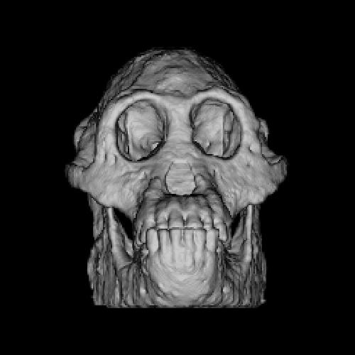
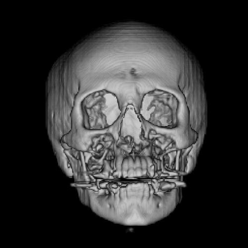
position. Below are two examples of volume renderings generated by the
provided demo executable.
How is this image created from a volume, given a specific viewpoint?
The mathematics and physics of volume rendering are beyond the scope
of this project; for our purposes a short answer suffices: we create
this image by simulating the light's journey (1) from the headlamp and
into the volume, and (2) out of the volume and back out into our
eye. Here is how we simulate each leg of this journey:
- For the first leg of the journey, we use a simple equation to
guess how brightly each cell glows; this equation uses not only the
value of the cell itself, but also the values of neighboring cells.
- For the second leg of the journey, we assume that light travels
along a single straight line, called a light ray, from each
cell towards the eye. Using this assumption, we now determine the
color of each image pixel as follows:
- We visit all cells behind a specific image pixel, in order,
moving along the light ray, starting from the cell closest to the eye,
and moving towards infinity. Initially, we assume that the ray color
is pitch black.

- As we visit each cell, we brighten the color of the light ray
(this is called shading) by adding the glow of the cell. To
be precise, we use a more complicated formula, not mere addition,
which takes into account the cell's glow as well as the opacity of all
the cells we've visited so far.
- We finish by assigning the ray color to the image pixel.
This process is called ray tracing. An interesting feature of
this approach is that some cells need never be visited: if, as we
march along a ray, we realize that we've marched through some dense,
opaque cells, then we can stop, or prune, tracing - the light
generated by any cells behind the opaque ones will never reach the
eye!
Tracing rays through volumes represented via octrees is easy if we
exploit the following property of the tree: a ray which does not cross
(the cell corresponding to) a node cannot cross any of the (cells
corresponding to) its children.
Task 7 [30 points]: Design, implement, and document
OctreeTraceRay(), which traces a given ray through a
volume, using your computed octree representation. The provided
functions CellTraceRay() - executing in O(1) time and space
- and ShadeRay() will respectively handle ray/cell
intersection and ray shading for you.
Task 8 [4 points]: Give tight asymptotic upper bounds
on the time and space complexity of your ray tracing
algorithm, as a function of volume size L. Each call to
ShadeRay() may make six calls to
GetOctreeValue(); ignoring these calls,
ShadeRay() consumes O(1) time and space. Argue the
correctness of your claimed bounds. [2 points each.]
Task 9 [5 points]: Make sure your code for
OctreeTraceRay() is no slower than ours. No points will be
given if your code is buggy.
Task 10 [Extra Credit]: Make your code as fast as you
can; the faster it is, the more extra credit you'll get. No extra
points will be given if your code is buggy. We will weigh most heavily
performance improvements for OctreeTraceRay().
Hints
Formulas
The average A and variance V of n numbers x1
... xn are
| A
| =
| ( x1 + ... + xn ) / n
|
| V
| =
|
( x12 + ... + xn2 -
n A2 ) / ( n-1 )
|
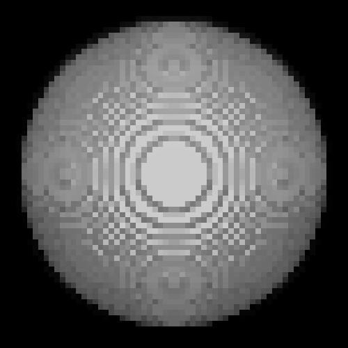
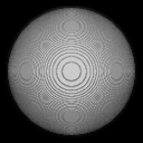
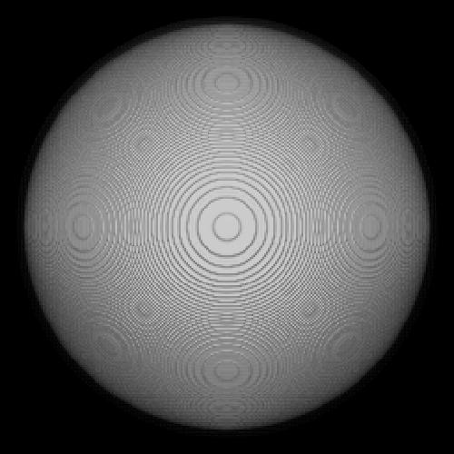
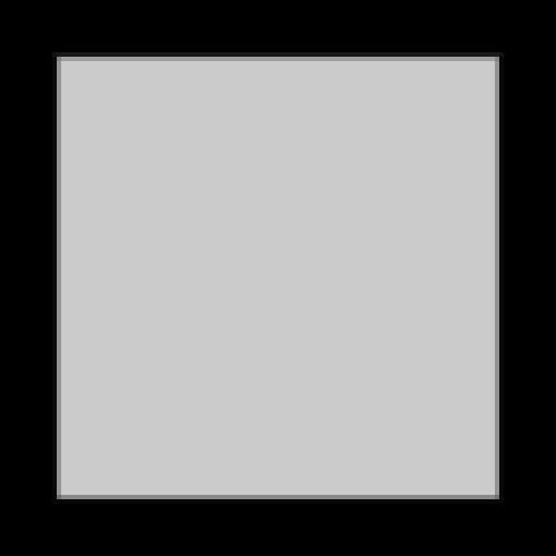
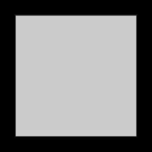
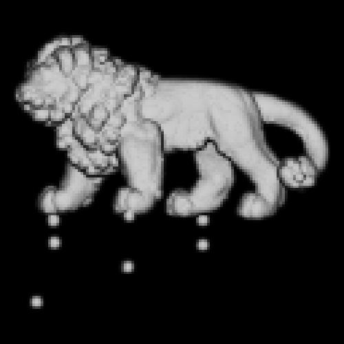
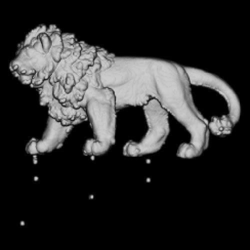
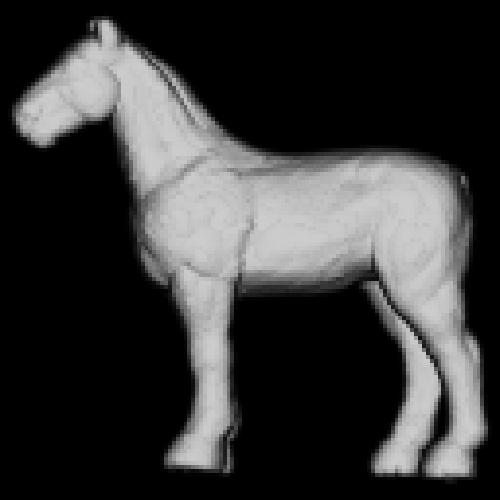
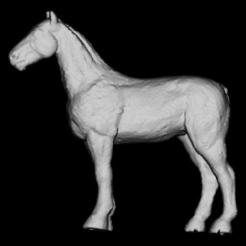
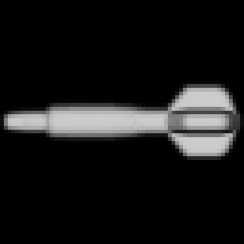
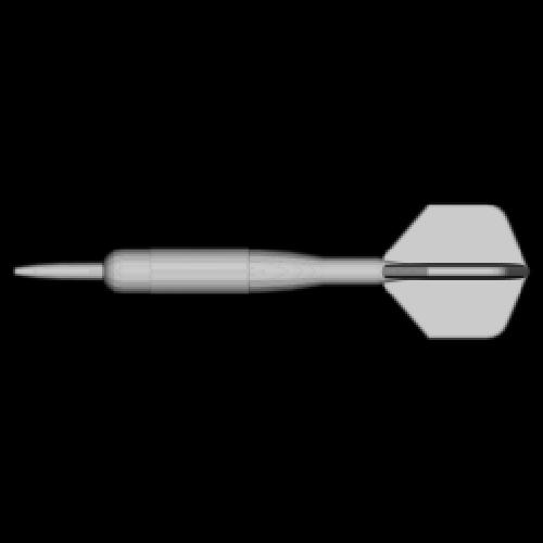
Catalog of demo volumes
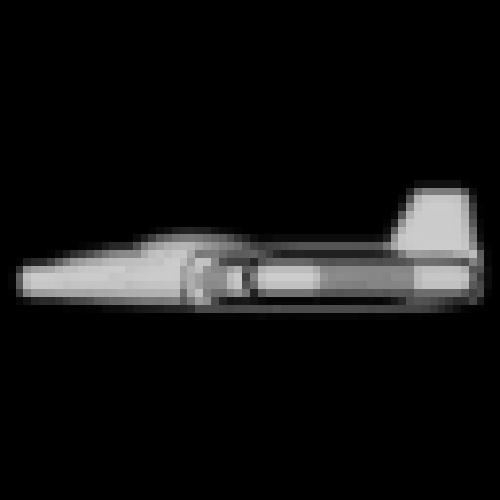
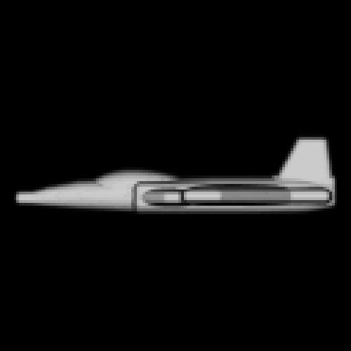
Below are sample renderings of selected demo volumes we provide, all
generated from a frontal viewpoint. All demo volumes are available in
the subdirectory data of the project directory. Our file
naming scheme consists of the volume name, all in lowercase, followed
by L, and ending with .vol.gz; for example,
sphere256.vol.gz.
Two demo volumes are not shown below: these are the orangutan (volume
name: "orangutan") and human ("human") heads shown earlier; these are
only available at the highest resolution (L=256).
| Volume Name
| L=64
| L=128
| L=256
|
| Sphere
|
|
 |
|
| Box
|

|

|

|
| Lion
|
|

|

|
| Horse
|
|

|

|
| Dart
|

|
|

|
| Plane
|

|

|
|
Demo movie
If we generate a collection of volume renderings of the same volume
but from slightly different viewpoints, the result is a movie! Here is
an example: a 1.5MB MPEG movie of
the horse demo volume, generated by rotating the viewpoint about the
volume.
Further information
For more information on octrees, we recommend the following sources;
the first two are on reserve at the Mathematical
and Computer Sciences library:
- Samet, Hanan. The Design and Analysis of Spatial Data
Structures. Addison-Wesley: Reading, MA, 1990.
QA76.9.D35.S26 1990
- Samet, Hanan. Applications of Spatial Data Structures:
Computer Graphics, Image Processing, and GIS. Addison-Wesley:
Reading, MA, 1990.
QA76.9.D35.S25 1990
- Foley, James D., Andries van Dam, Steven K. Feiner, and John
F. Hughes. Computer Graphics: Principles and
Practice. Second Edition, in C. Systems Programming
Series. Addison-Wesley: Reading, MA, 1996.
T385.C5735 1996
For more information on volume rendering, we recommend the following
sources; the first is available on-line, and its first chapter
contains an excellent introduction to the theoretical foundations of
volume rendering:
- Lacroute, Phil. Fast Volume Rendering Using a Shear-Warp
Factorization of the Viewing
Transformation. Ph.D. Dissertation. Technical Report
CSL-TR-95-678, Stanford University, Stanford, CA. 1995.
- Kaufman, Arie, Daniel Cohen and Roni Yagel. Volume
Graphics. Graphics. July 1993. 26(7): 51-64.
- Elvins, T. Todd. A Survey of Algorithms for Volume
Visualization. Computer Graphics. August
1992. 26(3): 194-201.
Finally, for volume rendering using octrees, you may consult the
following source: Levoy, Marc. Efficient Ray Tracing of Volume
Data. ACM Transactions on Graphics. July,
1990. 9(3): 245-261.
© 1998 Apostolos Lerios