Light Field Compression using Wavelet Transform and Vector Quantization

Li-Yi Wei
EE372, Winter 1997

Abstract

Image based rendering based on light fields offers interactive frame rate that's unachievable by traditional geometry based rendering techniques. However, the requirement for a huge amount of images causes problems both in mass storage and in memory management. In order to make light fields feasible even in low end computers we have to reduce the data size. This project suggests that by using wavelet transform and vector quantization we can achieve pretty high compression ratio with minimun degradation in rendering quality.

1 Introduction: Light Fields, Wavelets and Vector Quantization

1.1 Light Fields and Image Based Rendering

In traditional image synthesis techniques, we find physical models for the objects and simulate light reflections among them to generate the final image. The problem with this approach is that (1) We need accurate models for the objects, and sometimes it's hard to find out the models (2) The rendering time is prohibitive since we need to simulate zillions of light rays to get a noise free picture. In image based rendering, we pre-render or capture several images for the objects and render the final image by re-sampling those pre-aquired images. By doing so we can avoid the problem of object modeling and rendering complexity. Light Field is a image based rendering technique lead by Professor Marc Levoy and Pat Hanrahan in Stanford Computer Graphics Group. For people familiar with signal processing, light fields could be treated as 4D signals. For more information about light fields, please see [Levoy 96].

Although light fields could be rendered in real time even in personal computers, the amount of images required to represent a single object is pretty large. If we can't cache the required working set in memory during rendering, we will suffer from disk-swap operations and the iteractivity will be undermined. In order to reduce the data size and cache only the necessary working set in memory, we have to use some clever compression techniques. The requirements for light field compression would be:

• High compression ratio and low distortion.
• Random and real-time decoding.
• Hierarchy and multi-resolution structures so that we can cache only the necessary data set and render in a progressive fashion.

1.2 Wavelet Transform and Vector Quantization

2 Algorithm Overview

2.1 Encoding

(1)Wavelet transform: decompose the light field slabs into different subbands.

(2)Tree structured VQ: build separate binary VQ trees for different subbands using greedy split tree method.

(3)BFOS pruning: prune the trees back using BFOS algorithm

(4)Bit allocation: Use BFOS algorithm to do the bit allocation among the trees of subbands

2.1 Decoding

(1)Table look up: use table look up to get the subbands from the codebooks.

(2)Inverse wavelet transform: compose the original signal from the subbands.

2 Wavelet Transform

[Antonini 92] uses biorthogonal tensor-product wavelets to decompose images into subbands and VQ them separately. Biorthogonal wavelet filters have linear phases and short impulse responses so that we can do the convolution quickly while avoiding distortion. They decompose the images into 4 subbands( LL, LH, HL, HH ) and decompose only the LL component further until the desired depth is achieved. Then they use VQ to compress each subband using different bit-rates depending on the perceptual importance of each subband. The reported compression ratio and image quality is pretty good.

In compressing the light fields, we can use similiar approach. We can decompose each 4D light field signal into 16 subband and only decompose the LLLL subband further until the desired depth is reached. We have to pass through 4 levels of filter banks now to get 16 subbands out of one signal instead of 2 levels as in 2D image decomposition. We can plug in different filter banks to see the their performance in terms of computation time and image quality.

2 Tree Structured VQ

[Levoy 96] uses VQ compression followed by Lempel-Ziv coding to compress light fields. The VQ they used is ordinary GLA VQ. Because of the size of the light field is so large the training percentage could be only about 5%. In order to be able to have higher training percentage I decide to use binary tree structure VQ. The codewords won't satisfy the Lloyd optimality conditions in tree structure VQ but we can run much larger training sets.

The algorithm is as follows:

(1)Let the tree contains only the root node

(2)Assign all the training sets to the root node and calculate the codeword for root
( which is the centroid of all the training vectors )

root->trainingset = all training vectors;
root->codeword = centroid(root->trainingset);
root->distortion = distortion(root->codeword, root->trainingset);

(3)Split the node with most partial distortion until the desired number of codewords is achieved

current_num_codewords = 1;
while( current_num_codewords < max_num_codewords )
{
max_distortion_reduction = very small;
/* find out which leaf node to split */
for( each leaf_node )
{
/* split the node */
codeword1 = leaf_node->codeword;
codeword2 = leaf_node->codeword + eplison;
/* Use GLA algorithm to find the codewords for the training set */
GLA(codeword1, codeword2, leaf_node->trainingset);
leaf_node->left->codeword = codeword1;
leaf_node->right->codeword = codeword2;
for(each training_vector in leaf_node->trainingset)
{
if( distance(training_vector, leaf_node->left->codeword) < distance(training_vector, leaf_node->right->codeword) )
{
leaf_node->left->trainingset <- training_vector;
}
else
{
leaf_node->right->trainingset <- training_vector;
}
}
leaf_node->left->distortion = distortion(leaf_node->left->codeword, leaf_node->left->trainingset);
leaf_node->right->distortion = distortion(leaf_node->right->codeword, leaf_node->right->trainingset);
current_distortion_reduction =
leaf_node->distortion*size(leaf_node->trainingset)-
leaf_node->left->distortion*size(leaf_node->left->trainingset) -
leaf_node->right->distortion*size(leaf_node->right->trainingset);
leaf_node->left = leaf_node->right = NULL;
if( current_distortion_reduction > max_distortion_reduction )
{
max_distortion_reduction = current_distortion_reduction;
node_to_split = leaf_node;
}
}
/* the way split() works is exactly as the content of the for loop above */
split(node_to_split);
current_num_codewords++;
}

3 BFOS Pruning

The codeword tree built in tree structured VQ phase is locally greedy so that it may not be optimal. [Chou 89] use clever ways to find trees that lie on the convex hall among all the trees on the distortion-rate curve.

The algorithm is as follows:

(0) Initialization

Given:
A training sequence of N vectors
A tree-structured codebook constructed in tree structured VQ phase
for(each node in the tree)
{
node->d = 0;
node->count = 0;
node->delta_d = 0;
node->delta_r = 0;
if( node is a leaf )
{
node->lambda_min = infinity;
}
}

(1) Encode each training vector, updating d and count for each node

for( each training_vector )
{
root->d = root->d + distance(root->codeword, training_vector);
root->count = root->count + 1;
t = root;
while(t is an internal node)
{
d_left = distance(t->left->codeword, training_vector);
d_right = distance(t->right->codeword, training_vector);
if( d_left < d_right )
{
t = t->left;
t->d = t->d + d_left;
}
else
{
t = t->right;
t->d = t->d + d_right;
}
t->count = t->count + 1;
}
}

(2) Calculate delta_d and delta_r for all internal nodes

for( each internal node t )
{
t->delta_d = (t->left->d + t->right->d - t->d)/N;
t->delta_r = t->count/N;
}

(3) Evaluate root->d, root->r

root->d = root->d/N;
root->r = 0;

(4) Use a post-ordered traversal to calcualte delta_d and delta_r for each node

t = root;
repeat
{
while(t is an internal node )
{
t = t->left;
}
while(t is an internal node )
{
t = t->parent;
t->delta_d = t->delta_d + t->left->delta_d + t->right->delta_d;
t->delta_r = t->delta_r + t->left->delta_r + t->right->delta_r;
t->lambda = -t->delta_d/t->delta_r;
t->lambda_min = min(t->lambda, t->left->lambda_min, t->right->lambda_min);
}
if(t != root)
{
t = t->parent->right;
}
}
until(t == root)

(5)Prune:

r = root->r + root->delta_r;
d = root->d + root->delta_d;
while( root->lambda_min < infinity )
{
t = root;
while(t->lambda > t->lambda_min )
{
if( t->left->lambda_min == t->lambda_min )
{
t = t->left;
}
else
{
t = t->right;
}
}
delete all descendents of t from the tree structure
delta_d = t->delta_d;
delta_r = t->detla_r;
t->lambda_min = infinity;
while(t != root )
{
t = t->parent;
t->delta_d = t->delta_d - delta_d;
t->delta_r = t->delta_r - delta_r;
t->lambda = -t->delta_d/t->delta_r;
t->lambda_min = min(t->lambda, t->left->lambda_min, t->right->lambda_min);
}
d = d - delta_d;
r = r - delta_r;
write tree structure, d, r
}

4 Bit Allocation

After we get a forest of BFOS trees, we have to decide which tree should be used to encode each subband of signals. We can use BFOS algorithm again to do the bit allocation.

The algorithm is as follows:

(1) Given the trees generated in BFOS Pruning phase, and put trees of the same subband in the same class( they corresponds to a sequence of trees lie on the convex hall of the rate distortion curve )

(2) Calculate for each class n all possible values of the slope function

s(v_n, k_n ) = (r_n(v_n) - r_n(k_n))/(d_n(v_n) - d_n(k_n));
with d_n(v_n) < d_n(k_n), where r_n(v_n) and d_n(v_n) are the rate and distortion, respectively, of the nth quantizier under the bit assignment v_n, and find for each class the quantizier for which s(v_n, k_n) is maximal. Note that s(v_n, k_n) is the ratio of the change in rate to distortion between two bit assignments, v_n and k_n, which is exactly the reciprocal of lambda in the BFOS algorithm.

(3) Determine the class for which the maximum s(v_n, k_n) is the largest and assign to this class the quantizier for which this maximum is obtained.

(4) Calculate the new rate R and the new distortion D and check if they are sufficiently close to the desired bit rate or the desired distortion; if so, then stop the algorithm.

(5) Repeat (2), (3) and (4), but do (2) only for the class to which the new quantizier is assigned( the other values have not changed ).

5 Result

The following shows the result of compressing light fileds using different wavelets and codebook sizes. The spline wavelet I used is as follows:

n	-4	-3	-2	-1	0	+1	+2	+3	+4
(1/sqrt(2))h(n)	3/123	-3/64	-1/8	19/64	45/64	19/64	-1/8	-3/64	3/12
(1/sqrt(2))H(n)	0	0	0	1/4	1/2	1/4	0	0	0

Where h(n) is the low pass filter for analysis, H(n) is the low pass filter for synthesis.

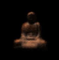
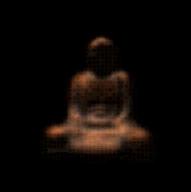
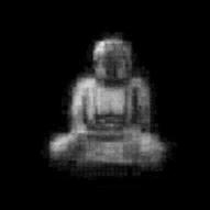
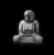
Each of the light fields below is decomposed via wavelet transform into 16 subbands, and each subband is trained and coded using a different codebook. The total size of the codebooks for each light field file is fixed and the bit allocation is determined by BFOS algorithm.

0 How to visualize the light fields

(1) Download the light field viewer
(2) Download my uncompress executable(only for SGI machines)
(3)Click on the icons below to download the compressed light field file
(4)Use my uncompress executable to uncompress them
(5)Use the light field viewer to see the uncompressed light fields

or

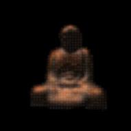
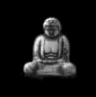
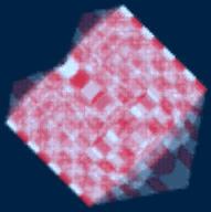
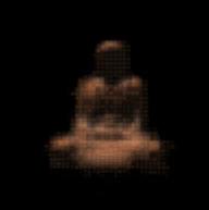
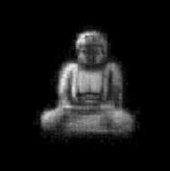
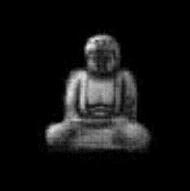
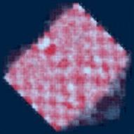
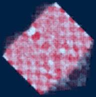
you can just click on the icons below to see the snapshots for the light fields

1 Original light fields

Golden Buddha	White Buddha	Checkcube

file	Golden Buddha	White Buddha	Checkcube
original size	16793216	37764736	1785470

2 Golden Buddha compressed using Haar wavelets with different number of codewords

The tile sizes u v s t are: 2 2 2 2 for the following light fields

1024 codewords	2048 codewords	4096 codewords	8192 codewords

The sizes of the compressed Golden Buddhas are as follows:

codewords	1024	2048	4096	8192
size	547629	824114	1399630	2480996
size after gzip	166575	283981	505827	912358

3 White Buddha compressed using Haar wavelets with different number of codewords

The tile sizes u v s t are: 2 2 2 2 for the following light fields

1024 codewords	2048 codewords	4096 codewords	8192 codewords

The sizes of the compressed White Buddhas are as follows:

codewords	1024	2048	4096	8192
size	902220	1196640	1835129	2957453
size after gzip	227558	363163	612267	1057119

4 Checkcube compressed using Haar wavelets with different number of codewords

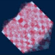
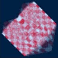
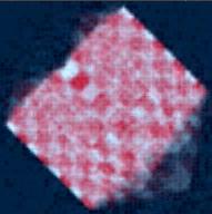
The tile sizes u v s t are: 1 1 2 2 for the following light fields

512 codewords	1024 codewords	2048 codewords	4096 codewords

The sizes of the compressed Checkcubes are as follows:

codewords	512	1024	2048	4096
size	178880	203473	280096	396897
size after gzip	50457	80982	118163	175055

5 Checkcube compressed using spline wavelets with different number of codewords

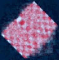
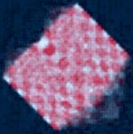
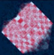
The tile sizes u v s t are: 1 1 2 2 for the following light fields

512 codewords	1024 codewords	2048 codewords	4096 codewords

The sizes of the compressed Checkcubes are as follows:

codewords	512	1024	2048	4096
size	178829	212680	280135	387235
size after gzip	56863	85951	147624	247622

6 Discussion and Future Research

From the above results we can see that by combining wavelet transform and tree structured VQ we can have hight compression ratio while maintaining the light field quality. Haar wavelet is generally not a good idea in applying to image compression but it seems to work pretty well for compressing light fields. By comparing the checkcubes compressed using Haar wavelet and spline wavelet we can see that in low bit rate case, the spline wavelet will smear out the boundary of the checkcube more than the Haar wavelet. One reason that Haar wavelet is not bad is that the light field viewer will do uv or st interpolation during rendering. Another advantage of Haar wavelet is that the computation is much simpler. For wavelet support of size n, the 4D tensor product of that wavelet will have support size n^4, which is 16 for Haar wavelet but 6561 for the spline wavlet I use. Because we need to render the light field in real time the time saving by Haar wavelet is very important.

In project we can see that wavelet transform followed by VQ is also very suitable for compressing light fields hierarchically. During rendering, we can swap in the wavelet coefficients in different hierarchies depending on their perceptual importance and viewing parameters. If we have enough coherence between successive frames the inverse wavelet transform we need to do should be small enough to maintain interactive frame rate. However, We will need clever caching strategies to decide how to cache the wavelet coefficients in memory so that we do not blow up memory easily. I will keep on researching how to render directly from wavelet-transformed-VQ-compressed light fields in real time under huge data sizes and constrained computing enviroment.

References