CS 223B Project: Color Edge Detection Program Analysis
Analysis and Parallelization Study
Program Flow
|
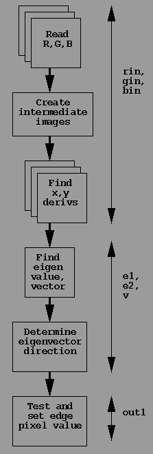
Pictured to the right is a diagram of the program flow. The arrows at
the far right indicate the temporary files involved in that particular
step of the process.
The implementation page describes
the program flow pictured at right; it will serve as a basis for our
discussion of possible parallelization of this program.
The parallelism in this program is present in several forms:
- red, green, and blue processing in parallel;
- rows of images processed in parallel;
- individual pixels within the rows processed in parallel.
We can also note that the lifetimes of many of the intermediate images
do not overlap; for clarity, those images have been kept separate as
to their function, but for efficiency, those images should be reused.
The memory storage for a single image, 512x512 with floats
representing intensity is considerable (1 megabyte on systems with a
32-bit representation for floats).
|

|
Loop structure
The loops in our program are two-level. The first level is a loop over
all the rows of the image, looping from the first valid y row to the
last. The second level is a loop over x for each pixel, from the first
valid x pixel to the last.
The current implementation sets three pointers in the loop for each
image (3 images [red, green, blue] in the derivative loop, 1 image in
the edge loop); one pointer for the current row, one pointer for the
row above the current row, and one pointer for the row after the
current row. The cases in which one of those pointers does not point to
a valid row (i.e. the row before the top row, and the row after the
bottom row) are correctly handled by the image library.
Our implementation loops through y, then x, and for each pixel
location calculates red, green, and blue. This loop structure is quite
simple and understandable but would absolutely clobber the cache on
each iteration, since the red, green, and blue cache lines would
likely map to the same cache location. A smarter organization would be
to loop through all colors at the top level, then y, then x.
Cache analysis
This code, like many scientific codes, suffers from poor cache
performance. Sequentially marching through a large array of values
will lead to no temporal locality in cache accesses, and spatial
locality only to the extent that adjacent pixels are stored in the
same cache lines.
Because the loops do not revisit their computed values (in the same
loop, although a combining of loops would change this), the temporal
cache locality is unimportant. However, a more sophisticated caching
strategy could aid in spatial locality.
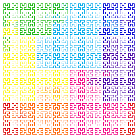
 A Hilbert curve (pictured at right) is a space-filling curve that
takes a minimum travel distance to complete traversal of the
curve. One advantage of using a Hilbert curve is the increase in
spatial locality given an intelligent cache organization.
That cache organization requires that data is stored not in row order
but instead in cache blocks, where a single cache line contains data
for a m-by-m block of pixels instead of a n-by-1 row. For example, a
64-byte cache line with 4-bit floats would have a 4-by-4 block of
floats instead of a 16-by-1 row.
Using the above example (16 floats per cache line) we can see that a
blocked scheme has a lower miss rate per access than a row scheme for
any random access. These results are shown in the table below. The
gains in temporal locality (not calculated) by traversing a Hilbert
curve are greater still.
| Strategy | Expected Number of Blocks Referenced |
| 16-by-1 row | 3.375 |
| 4-by-4 block | 2.25 |
The arithmetic to calculate memory offsets is more complicated for a
blocked cache method, but is far less significant than the cost of
additional cache misses. Sun's Visual Instruction Set (VIS) has array
instructions which perform this arithmetic transparently, so even the
arithmetic cost is eliminated. It is also slightly more complicated
to traverse the Hilbert curve than to page through the nested loops.
It is unlikely that any cache would be so small so as to have
conflicts between adjacent rows in the image. However, to avoid this
situation we should pad the ends of our rows with a prime number of
cachelines of blanks so that adjacent rows do not map into the same
lines of the cache. The disadvantage to this strategy is the
additional storage space necessary.
Fine-grained parallelism
Any gains using fine-grained parallelism (by using multimedia
instruction sets) would come at the expense of data
precision. Currently we use floats to represent each of the red,
green, and blue intensity values for each pixel. This precision is
probably greater than necessary; 24-bit color is certainly sufficient
for vision applications, meaning only a single byte should be
necessary to represent a single color's intensity value. It is likely
that noise in any acquired image would be more significant than the
loss of precision.
Cutting the precision from float to byte cuts the memory footprint
into a quarter its previous size. This will increase cache hit rates
by reducing capacity cache misses, as well as reduce the number of
pages required.
With a reduction in size to a single byte the parallel instructions of
multimedia instruction sets can greatly reduce the number of
instructions necessary to complete the pixel operations. Two options
are available for encoding the data:
- We could encode the neighbors of a pixel as well as the pixel
itself in a given word. This approach would have the best cache
behavior as only a single word per pixel is necessary, and operations
on that pixel could be completed and the pixel discarded, thus
eliminating cache conflict misses. However, multimedia instructions
generally operate between disparate words as opposed to within words,
making those computations difficult. Also, each datum would be encoded
9 times, both as a pixel value and 8 times as a pixel's neighbor
value. Finally, encoding 9 pixel values in one word is problematic;
even the densest words, associated with 64-bit machines, only pack 8
bytes into a single word.
- A better approach would be to encode 8 neighboring pixel values
into a single word. A 4-by-4 word cache block would thus have 32
pixels in the horizontal direction and 4 in the vertical direction
(which might lead to a conclusion that a 2-by-8 cache block would be
superior). Eight operations could be performed in vector fashion on
each cache line at the same time. The most efficient computation would
probably require replicating the data 3 times, because the kernels are
3 pixels wide; shifting twice and redoing the computation is probably
a better alternative.
Convolution
No commercially available multimedia instruction set contains any
convolution operators; these are strictly the domain of digital signal
processors at this time. Commercial microprocessors are moving towards
DSP functionality, however; SGI's new MDMX offering includes a 192-bit
accumulator, a size that was previously only in DSPs. Intel's Andy
Grove frequently speaks about his 'NSP' or Native Signal Processing
initiative, an effort to move DSP functionality into the microprocessor.
This application is clearly well suited to a convolution operator. The
first major loop implements difference functions for derivatives; the x
derivative, for example, could be implemented with the operator
      0   0    0
    -0.5  0   0.5
      0   0    0
and the y-derivative would use a similar operator rotated 90 degrees.
It is also conceivable that a convolution operator could be used to
execute the edge thinning step in the second main loop. The
computation is murkier, however, since the eigenvector direction is
also involved, and it is unclear that a simple convolution could
do the necessary filtering. This step is not a good candidate for a
general-purpose instruction.
The major roadblocks to the use of convolution operators would be
- the difficulty of efficiently coding an operator into registers;
- squeezing all the computation involved in computation into a
reasonable number of cycles.
Return to project overview.

 A Hilbert curve (pictured at right) is a space-filling curve that
takes a minimum travel distance to complete traversal of the
curve. One advantage of using a Hilbert curve is the increase in
spatial locality given an intelligent cache organization.