The provided executable executes only on Silicon Graphics workstations equipped with the execution-only-environment (eoe) of Open Inventor (the development environment is not required). For those interested in porting scurvy to other platforms, the source code is also available in tar archive format; use tar xf scurvy.tar to unpack the archive. This source code was developed on a Silicon Graphics workstation equipped with the Open Inventor development environment. A Linux port is also available, contributed by Björn Leffler (bleffler@kth.se).
We provide no support for scurvy.
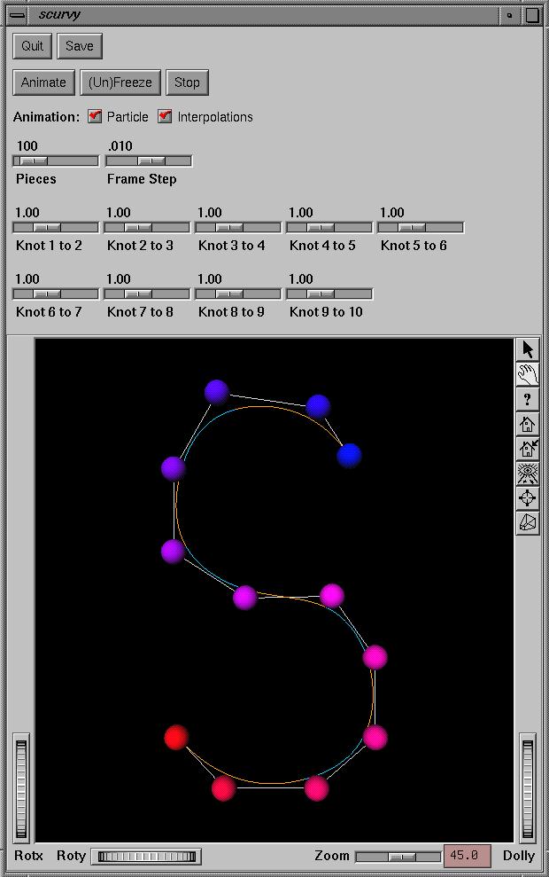
The colored spheres mark the de Boor points of the curve. The color of the spheres indicates the order of the de Boor points: the first point is blue, and the last is red, while intermediate ones have colors in-between blue and red. The white polyline connecting the spheres is the control polygon of the curve; along with the spheres' coloring, it identifies the ordering of the de Boor points.
The spheres can be interactively moved by a click-and-drag interface: but first press the small arrow button on the side of the main window. Also, the viewpoint may be interactively changed: press the small hand button first. These aspects of the user interface are provided by the Open Inventor toolkit, documented on-line: just press the small "?" button.
When a sphere is selected, some of the curve segments are drawn in yellow or green, instead of the customary orange or cyan (respectively). These highlighted segments are the ones whose shape will change if the selected de Boor point is moved.
The spacing between the spline knots can be interactively modified using the sliders labeled "Knot i to i+1". These sliders allow a minimum spacing of 0.1, thus disallowing any changes in the multiplicities of the knots.
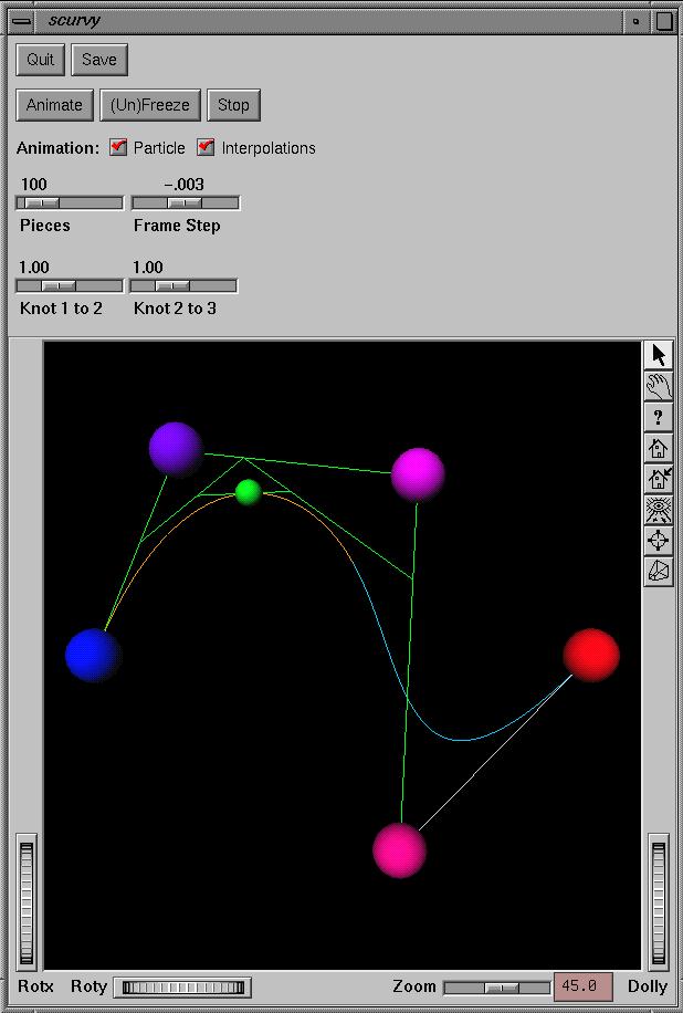
Pressing the "Animate" button makes a green sphere appear and travel along the curve. That is, the equation of the curve is perceived as a formula producing the location of a particle (the green sphere), given the simulated time as parameter.
The animation starts with the particle placed on the first de Boor point. It ends when either the "Stop" button is pressed, or the particle passes the last de Boor point while moving forward (in simulated time), or the first de Boor point while moving backward. It is possible to freeze an on-going animation by pressing the "(Un)Freeze" or "Animate" buttons; to resume the animation, press one of these buttons a second time.
The speed of the particle's movement is controlled by the "Frame Step" slider. This slider sets the amount by which the simulated time is advanced between successive animation frames. Positive and negative values are allowed, effecting forward and backward movement.
As the particle travels along the curve, a collection of green lines appears; see the example screen above. These lines connect points that were interpolated by the de Boor algorithm while computing the particle position.
The visibility of the interpolation lines and the particle can be independently changed using the "Animation" check-boxes.
The parameter file contains a complete specification of a B-spline curve. As we saw earlier, some of the spline parameters can be interactively modified during scurvy's execution. A new parameter file, containing the modified spline parameters, can be generated by pressing the "Save" button. In order to compose parameter files by hand, here is the description of their format, followed by an example:
# The degree d of the spline, i.e. the degree of each of the
# polynomial curves that comprise the spline.
#
# d must be an integer greater than or equal to 1.

3

# The number n of the spline's knots. Alternatively, the number of
# spline segments (i.e. adjacent polynomial curves) augmented by one.
# We consider knots to be distinct numbers which may appear multiple
# times in a knot sequence; n should ignore these multiplicities.
#
# n must be an integer greater than or equal to 2.

4

# The values of the spline's knots.
#
# n real numbers in strictly increasing order should be listed in
# separate lines.

0
1
2
3

# The multiplicities of the interior knots, i.e. all knots except the
# first and last one. The multiplicities of the first and last knot are
# both automatically set to d.
#
# n-2 integers between 1 and d+1 should be listed in separate lines.

1
1

# The de Boor points of the spline.
#
# The tab-separated x, y, and z coordinates of the first point should
# be followed on the next line by the coordinates of the second point,
# and so on. Each coordinate is a real number. The coordinates of s+d+1
# points should be listed, where s is the sum of the multiplicities of
# the interior knots, i.e. the sum of the numbers in the previous field.

0.0	0.0	0.0
3.0	5.0	0.0
9.0	5.0	0.0
12.0	-5.0	0.0
18.0	-5.0	0.0
21.0	0.0	0.0
Permission to use, copy, modify and distribute this software for any purpose is hereby granted without fee, provided that the above copyright notice and this permission notice appear in all copies of this software and that you do not sell the software. Commercial licensing is available by contacting the author.
This software is provided "as is" and without warranty of any kind, express, implied or otherwise, including without limitation, any warranty of merchantability or fitness for a particular purpose.
Author: Apostolos Lerios.