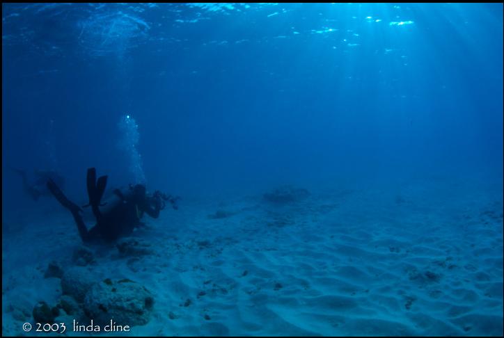
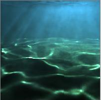
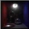
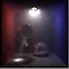
For our final project, we were interested in creating realistic underwater scenes, with beams of light and accurate light caustics on the sea floor. Our inspirations for the project stemmed from some incredible underwater pictures, shown below:
Our original proposal can be found here.
To implement the scene, we worked with PBRTs existing photon mapping and volume rendering code, and extended it to allow for photon mapping through participating media. In addition, we added a few optimizations to improve image quality:
For the project:
To implement photon mapping with participating media, we wrote an algorithm for photon map creating that ray marches through the scene for a given light. The algorithm first casts the ray, and checks if it intersects anything in the scene. This determines the ray's behavior in the event that the ray does not interact with a volume or a volume is not present. For each ray sampled from the light, the algorithm would first check if the ray hits the volume at any point. If it does, it divides the current ray into steps of constant size with jitter, and for each step through the volume, calculates whether the ray interacts with the medium for that step, using the cumulative distribution function in the Jensen paper. Upon interaction, a volume photon is added to the map for the current interaction point and light direction. Finally, it determines whether the interaction is an absorption, or scatter, and generates a new ray in a direction determined by importance sampling the phase function of the medium.
If the ray march proceeds without any interaction with the media, then the ray has either hit a surface in the scene or has exited the volume without hitting anything. If a surface was hit, then the direct/indirect/caustic maps are filled using standard photon map generation for surfaces. A new direction for the ray is determined by sampling the BSDF, and the process repeats. After three interactions or bounces, the ray has a 50% chance of termination via Russian roulette.
During the eye ray traversal stage, for each step, we added the contribution from inscattering by using the volume photon map. For a given point during a ray march, we did a lookup, with no final gather step. When using the surface photon maps, however, final gather was always used.
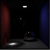
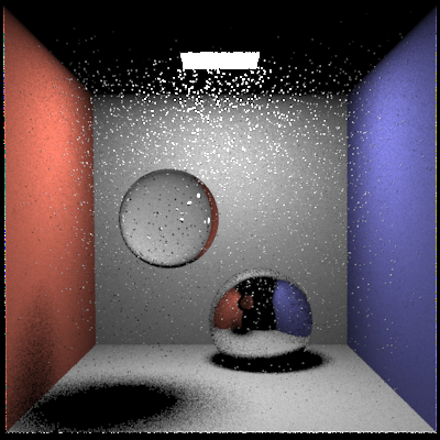
What rendering project would be complete without a few Cornell box images? We
created a Cornell Box scene file to initially test the modified photon mapping
algorithm. The Cornell box is nice in that it easily allowed us to compare our
images to existing images in the Jensen paper [1]. Below is an example image:
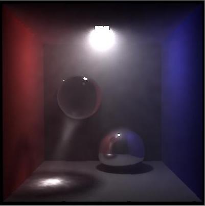
This image was rendered in 400x400 using a total of 1,040,000 photons, with 500,000 used for the volume and indirect maps, and 40,000 used for the caustic map. In all of our renders, we used final gathering for the surface photon map lookups.
While we used an isotropic scattering distribution for the final images, we also extended the pbrt language to handle anisotropic scattering for ray marches through the scene. To do this, we modified the core code to allow our ray marcher to generate samples according to the volumes phase function. We initially tried doing this by sampling over a uniform sphere, then weighting the resulting directions by the phase function for the given incident and new outgoing directions. However, this created artifacts, so we modified the code to importance sample the scattering direction based on the phase function.
Here are some images to demonstrate anisotropic scattering (note, the lack of
volume was due to a precompute alpha setting that was missing in our initial
images): 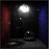
The first image is the result of g=0.8 before we modified the code to importance sample the phase function. The second image is the result after the modification. The third image shows isotropic scattering (ie g = 0), while the final image shows the scene at g = 1.
During the course of building the photon map, it became necessary to verify
the distribution of the volume photons in the scene. We used the cornell box
scene to create a visualization of the volume photon locations and color values.
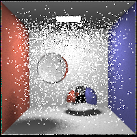
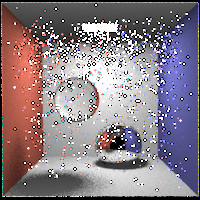
The first image is a high res visualization of where the volume photons end up. It was produced by dumping the volume photon map to a scene file, with each photon represented as a translated sphere. This scene file is then rendered without global illumination, but with the spheres indicating the location of the photons. The second image is a lower res version of the photons where each photon is given a uniform color to make the general distributions easier to see. The final image shows the spatial and spectral distribution of the photons in the scene, artificially brightened to make them easier to see. One thing to note is while the scene used includes a back wall for the cornell box, the photons being visualized are from a scene file without a back wall.
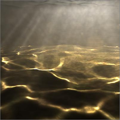
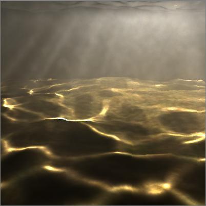
The underwater scene consists of a point light source 5 units about the water, slightly offset from the center of the water. The water and land are both implemented as height fields, using heightfield data from a previous assignment. The water and floor are 30x30 units, with a separation distance of 10 units between the water and the floor. The floor has a sand texture applied as well. The participating media was defined as a homogenous, isotropic volume, with an absorption sigma of 0.01, and a scattering sigma of 0.05.
The water was defined as a glass surface, with an index of refraction of 1.33, and with a transmission 'spectrum of 14%, 36%, 50% over the RGB to give the scene a deep blue color reflective underwater ocean colors.
In general, creating and setting up this underwater scene and the cornell scene took a huge chunk of time, especially with the long render times associated with ray marching through participating media.
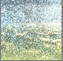
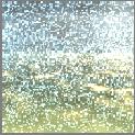
During rendering, we found that a fixed step size would introduce aliasing in the image in the form of clearly defined bands of intensity in the volume region. To counteract this, we added jittering to the ray marching step for both the photon gathering and lookup stage. In our algorithm, the ray would march a random distance between .5x and 1.5x the fixed step size.
Below are images showing before and after effects of the jittering algorithm. In the left image, there is obvious banding in the volume at the right side of the image. Introducting jittering effectively removed this banding, as shown in the right image, while keeping the god rays sharp and focused.
We were considering simulating the sky using a bright white directional light to simulate the sun and adding an environment map to try and capture the blue sky. To handle this situation without introducing excessive amounts of noise we changed the uniform sampling between the lights to use importance sampling to choose which light to sample. Unfortunately doing this actually increased the visual noise, because most of the time the darker sky was not sampled, but when it was it was very strongly weighted, so that some pixels were bright blue while the rest were unaffected. Below are pictures showing such a scene with and without importance sampling being used to choose which light to sample. For each pair, the first image is with 16 samples per light and the second is with 64 samples per light.
16 Samples: 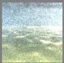
64 Samples: 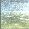
We ran into problems during the rendering process with pbrt causing crashes for certain scene files. We isolated the problem to a classmate's heightfield code, which he graciously allowed us to use after we found rendering issues with our existing heightfield code. Despite extensive investigation, we couldn't find the cause of the problems in the code. As a result, while all of the images of the underwater scenes used this code, we can't guarantee that the render will work for every scene file that uses a height field. Scene files that don't use height fields, however, seem unaffected.
Below is our result:
Here is the final scene with blue tints. During the intermediate image
creation phase, we primarily used a white light with water that refracts the
light in equal frequencies. Our final image changes the refraction
characteristics of the water to transmit more of the blue light. 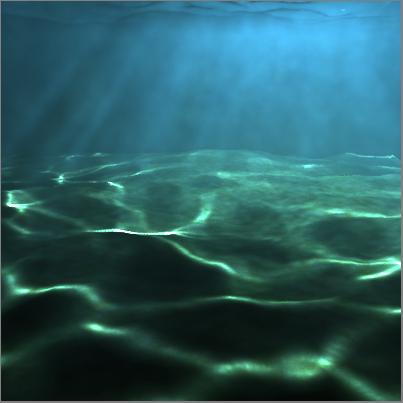
A large version of the scene can be found here:
The image above shows some nice caustics on the ocean floor, and the murkiness of the water. In addition, a number of "god rays" are evident in the render, with the rays accurately originating from the source of the light, which is above the water, and to the right and front of the camera.
The source code for our project can be found here. We had to modify a few of the core classes to get the functionality we wanted. In addition, we used classmate Mathieu Bredik's heightfield code with his permission, and that is included in the code as well.
The scene files used to render the final image can be found here. Also included are some of the cornell box and white light test scene files.
In general, we were very pleased with the results. Particularly, the caustics on the floor and the godrays show up quite prominently in the image. Though insanely frustrating at times, we both learned a lot and had a lot of fun in the process.
[1] "Efficient Simulation of Light Transport in Scenes with Participating
Media using Photon Maps"
Henrik Wann Jensen and Per H. Christensen
Proceedings of SIGGRAPH'98, pages 311-320, Orlando, July 1998
[2] Realistic Image Synthesis using Photon Mapping
Henrik Wann
Jensen
[3] "Rendering Natural Waters."
Simon Premoze, Michael Ashikhmin.
http://www-graphics.stanford.edu/courses/cs348b-competition/cs348b-01/ocean_scenes/ocean.pdf
[4] Color and Light in Nature: Second Edition
David Lynch,
William Livingston
[5] "A Practical Guide to Global Illumination using Photon Mapping
Henrick Wann Jensen
SIGGRAPH '01