|
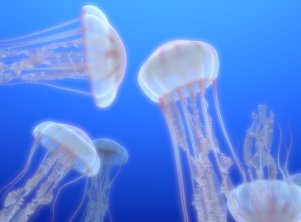
Inspired by striking photographs of sea nettles lit under ultraviolet light at the Monterey Bay Aquarium, our goal was to create an animated underwater scene containing jellyfish. Images of jellyfish proved to be an interesting subject to attempt to reproduce due to the intricacy of the creature's geometry, the presence of translucent surfaces that scatter light, and the beautiful appearance of the creatures when placed under particular lighting conditions. The photographs of jellyfish at the Monterey Bay Aquarium that served as the starting point for our project can be seen here. Our original project proposal sits here. Modeling
the Jellyfish |
 |
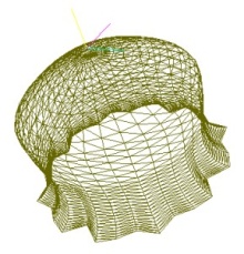 Each jellyfish is defined by small set of parameters and user specified
splines. A triangle mesh for each region of the jellyfish is constructed
from these inputs and fed to pbrt. The bell of the jellyfish is modeled by
lathing a Hermite spline around an axis of rotation defined by the
jellyfish's orientation. Hermite splines were chosen to give us the
ability to more carefully define the shape of the bell. Catmull-Rom
splines did not provide enough control since derivatives cannot be
specified. A second spline curve is used to govern the displacement of the
surface to create frills in the bell. All splines are reparameterized by
arc-length, resulting in a mesh containing triangles with roughly equal
area. The parameterization by arc-length also minimized the "sliding" of
geometry along the parameterized surface as the control points of the
spline curves were animated.
Each jellyfish is defined by small set of parameters and user specified
splines. A triangle mesh for each region of the jellyfish is constructed
from these inputs and fed to pbrt. The bell of the jellyfish is modeled by
lathing a Hermite spline around an axis of rotation defined by the
jellyfish's orientation. Hermite splines were chosen to give us the
ability to more carefully define the shape of the bell. Catmull-Rom
splines did not provide enough control since derivatives cannot be
specified. A second spline curve is used to govern the displacement of the
surface to create frills in the bell. All splines are reparameterized by
arc-length, resulting in a mesh containing triangles with roughly equal
area. The parameterization by arc-length also minimized the "sliding" of
geometry along the parameterized surface as the control points of the
spline curves were animated.
The Jellyfish's small tentacles are modeled as generalized cylinders. The backbone spline of the generalized cylinder is given by a Catmull-Rom spline whose control points are determined by the locations of particles in a mass-spring simulation discussed in part 2. Since it would be ackward to specify derivatives at each control point in this case, Catmull-Rom splines were used instead of Hermite splines. We used a technique given by Ken Sloan to avoid twisting of geometry when generating triangles for the surface of the tentacles.
The most difficult aspect of realistically modeling the jellyfish was reproducing the intricate geometry of the large inner tentacles. The tentacles are modeled as a long thin sheet whose central axis is defined by a Catmull-Rom spline. As done for the small tentacles, a coordinate system is obtained for each sample point on this spline. We then generate two splines f1 and f2 to define the displacement of the surface in the z direction (local coord system) at the edges of the tentacle. The height of the surface at intermediate points is then interpolated using a parameter that is quadratic in x. A cross-section view of a large tentacle is givne below.
Control points of f1 and f2 are generated via a random walk. This gave more pleasing results than a noise function. The x-distance between the edges of the tentacle is also determined by a random spline. Finally, the tentacle is given rotation by rotating the local coordinate systems at each sample point along the backbone spline. The change in this rotation between sample points is determined by yet another spline.
 The jellyfish is animated using a combination of keyframing and
simple simulation. The overall velocity of the jellyfish is determined by
a user specified Hermite spline. Parameterization by arc length is
required for animation splines to ensure uniform velocity over time.
The jellyfish is animated using a combination of keyframing and
simple simulation. The overall velocity of the jellyfish is determined by
a user specified Hermite spline. Parameterization by arc length is
required for animation splines to ensure uniform velocity over time.
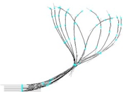
The bell animation is keyframed. The user specifies a set of Hermite splines to use as keyframes. Surprisingly, we found that given enough keyframes, linear interpolation of the keyframes was sufficient for visually pleasing results. They keyframe splines for the bell animation sequence are shown at left.
The control points of the small and large tentacle backbone splines are animated via a simple damped mass-spring particle system (we simulate a rope with stretch and bend springs, attached at one end to a point on the surface of the bell). Midpoint integration is used to time step the system.
To make the large tentacles appear less rigid, a turbulence field is generated using a combination of sin curves. Additionally, the edges of the large tentacles are purturbed sinusoidally with slightly higher frequency than the forces on the simulated particles. None of these effects have any physical basis, but yielding plausible animation results.
Jellyfish Surface Material
Out initial goal in rendering the jellyfish was to accurately model reflection, transmission and single scattering for thin surfaces. We implemented the model given in Hanrahan and Krueger's "Reflection from Layered Surfaces due to Subsurface Scattering." However, we found that reproducing the vibrant appearance of our reference photos using this model under plausible illumination was difficult.
Further discussion led to the realization that the dominant factor in the appearance of our reference images was the fluorescence of the jellyfish under ultraviolet illumination. Rather than try to model fluorescent materials and UV illumination in PBRT we made the simplifying assumption that the fluorescent term could be modeled as uniform volumetric light emission (for sufficiently uniform UV illumination). We thus extended our thin surface material model to account for light emission as well as scattering. Texture mapping the level of emission across the bell and tentacles allowed us to add variation to the surfaces and generate a convincing appearance.
The following images show our jellyfish surface model without texture mapping of the emissive color:


Volumetric Photon Mapping
Our implementation of volume photon mapping was based on two primary sources. The first was the PBRT code for photon mapping of surfaces, and the second was Henrik Wann Jensen's "Realistic Image Synthesis Using Volume Photon Mapping." The PBRT surface photon mapping already included code for shooting and storing photons in a k-d tree, as well as code for finding the N closest photons to a point and making a surface radiance estimate. Thus adding volumetric photon mapping was a matter of extending the photon shooting to include scattering and absorption, as well as adding ray marching and a volume radiance estimate to accumulate these photons for rendering.
During the shooting phase we take each photon ray (whether shot from a light source or scattered from a surface or volume element) and intersect it with the volume elements of the scene. We then estimate the average combined scattering/absorption cross section of the volume along the ray. Using this information we importance sample a "time to next interaction" with the volume. If a surface obstructs the ray before this next interaction then we use the standard PBRT codepath to handle the surface intersection. Otherwise we store the photon in an appropriate k-d tree and use the albedo of the volume to select between absorption and scattering
Our ray-marching implementation was achieved by extending the standard PBRT single-scattering volume integrator. This integrator already marched rays through the volume and estimated in-scattered radiance resulting from direct lighting. We extended this integrator by using the previously-stored photon maps to make radiance estimates at each point sample. Our photon map lookups added in-scattered radiance due to multiple volume scattering as well as light that had scattered from both surfaces and volumes. The following image shows how out volume integrator can correctly realize the volume caustic projected by a bright light source through a glass sphere:

We found, unfortunately, that our volumetric photon mapping implementation did not behave as expected in our underwater enviornment. Whether it was a result of our simplistic water surface geometry or a bug in our implementation, we were never able to reproduce the "shafts of light" that might be expected in a marine environment without giving our surface waves unrealistic amplitudes. This shortcoming might have been avoided had we given more time to correctness testing on the photon mapper, physically plausible water surface simulation, and correct scattering and absorption properties for marine water.
Furthermore, animating scenes with our photon maps led to objectionable temporal noise. Rather than increase the number of photons shot and used in our radiance estimates to drive down the noise (at a significant cost to rendering time) we chose to "bake" our photon map configuration on the first frame of animation and re-use that data for subsequent frames. This eliminated the temporal noise, leaving only spatial noise and implausible appearance as the remaining problems with our photon mapping.
The following images show some early results in our search for plausible and attractive underwater volumes:

Click on images to view high resolution versions.
 |
Jellyfish surrounded by a blue environment map swimming in a homogeneous blue volume. A bloom filter has been applied as a post process. Each jellyfish contains approximately 250,000 triangles.
Click here to view the high res tiff (3079K). Click here to view the animation (2927K). |

|
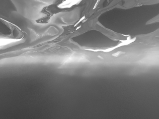
In this scene we use volumetric photon mapping to attempt to capture light scattering effects through the water. The water's surface is a 1000x1000 resolution heightfield. An optical manhole effect due to total internal reflection is visible behind the jellyfish. A bloom filter has been applied as a post process.
Click here to view the high res tiff (3079K). Click here to view the animation (1449K). |
 |
Jellyfish rendered against a black background to make the geometric detail of the surfaces more apparent.
Click here to view the high res tiff (3087K). Click here to view the animation (3311K). |
Project completed June 2004 by Kayvon Fatahalian and Tim Foley.