Khai
Weyn Ong (weyn@stanford.edu)
Spring 2002
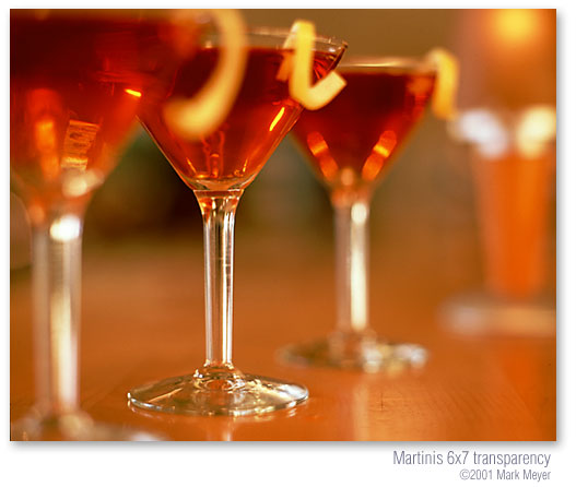
Original photograph
The aim of this project was to extend lrt to be able to render an image similar to the above photograph. This photograph, Martinis, was taken by Mark Meyer. Please visit his website http://www.photo-mark.com/ to view the rest of his fine portfolio.
The original project proposal can be found here.
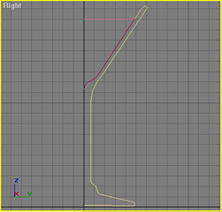 The martini glasses are modeled as surfaces of revolution. Each glass
is defined by three 2D contours - one each for the glass-air, glass-liquid and
liquid-air boundaries. These contours are defined by a series of connected
points and are entered into the RIB file as a new primitive -
MartiniGlassContour. Any modeling program can by used to obtain those contour
points. Intersection with the full 3D surface is calculated by treating each
adjacent pair of points as the defining points for a hyperboloid that is
centered about the vertical axis. The bounding boxes for these "strips" are
arranged hierarchically for accelerated intersection. Normals are interpolated
both in the longitudinal and latitudinal directions for smooth Phong shading and
more accurate intersection behavior. Defining the martini glasses in this way
make intersection much faster (and probably more accurate) than exporting a
large triangle mesh from a modeling program.
The martini glasses are modeled as surfaces of revolution. Each glass
is defined by three 2D contours - one each for the glass-air, glass-liquid and
liquid-air boundaries. These contours are defined by a series of connected
points and are entered into the RIB file as a new primitive -
MartiniGlassContour. Any modeling program can by used to obtain those contour
points. Intersection with the full 3D surface is calculated by treating each
adjacent pair of points as the defining points for a hyperboloid that is
centered about the vertical axis. The bounding boxes for these "strips" are
arranged hierarchically for accelerated intersection. Normals are interpolated
both in the longitudinal and latitudinal directions for smooth Phong shading and
more accurate intersection behavior. Defining the martini glasses in this way
make intersection much faster (and probably more accurate) than exporting a
large triangle mesh from a modeling program.
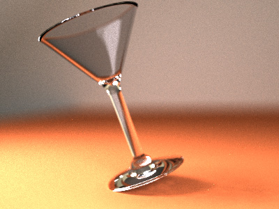
Two new materials were designed. The first is a more accurate model of glass which takes into account the Fresnel equations for determining how much light is refracted/reflected depending on the angle of incidence. The second is a special volumetric boundary material that also uses a Fresnel BSDF and stores information about the volumetric body it bounds (i.e. indices of refraction, scattering/absorption coefficient, scattering direction parameter for the Shlick phase function). This volumetric boundary is used for the glass-liquid and liquid-air interfaces.
 |
 |
|
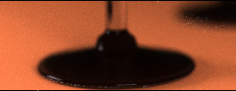
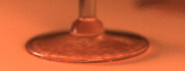
Glass without Fresnel scattering |
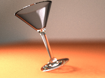
Glass with Fresnel scattering. Note the
characteristic darkening of the sides of the glass at low-incidence
viewing angles. Also note the more accurate caustics beneath the
base. |
Henrik Wann Jensen's photon mapping solution to the global illumination problem is the main extension made to the existing ray tracer. I made use of his photon map data structure to set up two photon maps - one for caustics and one for volumetric rendering. The caustics photon map is created by emitting photons from each light source stochastically and tracing them through the scene; photons that hit one or more specular surfaces before impinging on a diffuse surface are stored in the photon map. In this particular scene, most of the caustics contribution is directly under the bottom of the glasses. The table surface there is effectively hidden from direct illumination by the (transparent) glass base, and would be very noisy if we relied purely on monte carlo / path raytracing to sample the illumination. With the photon map, it is possible to estimate the incoming radiance by gathering photons in the immediate vicinity of the hit diffuse surface.
The number of photons emitted from each light souce is proportional to the power of the light source. This results in a photon map containing photons of approximately equal power (since the power of each photon is scaled down based on the number of photons emitted from the light source), giving better approximations in the photon gathering phase.
 |
 |
|
Without caustics |
With caustics |
Instead of modeling the liquid as a vacuous body, I used volumetric rendering to simulate the scattering effects of a participating medium. The volumetric body is homogeneous and is defined as the region within the boundaries of the liquid-air and liquid-glass surfaces. When a ray hits a volumetric surface, it is either reflected or refracted according to the Fresnel / Snell equations. If it is refracted into the liquid, a ray-marching procedure is used to gather the direct illumination incident on each differential segment of the ray. The incoming radiance is attenuated by the distance the incoming light ray travels within the volumetric body.
Multiple scattering (indirect illumination) is simulated with the aid of the second photon map - the volumetric photon map. This photon map is created by emitting photons from each light source and allowing them to interact with the volumetric body. The distance each photon travels in the volume before the next interaction is stochastically chosen according to the extinction coefficient of the medium. At each point of interaction, the probability of scattering vs absorption is given by the albedo, and the direction of a scattered photon is computed by importance-sampling the phase function. The Shlick phase function is used in this case. The photon is stored at each point of interaction after the first scatter (so that the direct illumination is not double-counted). Again, photons are approximately of the same power because Russian roulette is used instead of generating multiple descendent photons with scaled-down powers.
During the ray tracing phase, a spherical region about each differential ray segment is used to gather an irradiance estimate from the stored photons.
Defining the volumeric body as the region enclosed by boundary surfaces caused some problems with lrt's implementation of ray tracing. The usual epsilon hack meant that surfaces were sometimes missed because they were too close to the starting point of the ray. This could occur where the volumetric surfaces are very close to each other (e.g. at the edge of the top surface of the liquid, where the liquid-glass and liquid-air boundaries meet) or when a photon happens to interact with the medium at a point close to the boundary (and then "misses" the boundary on its next ray out). I could see no easy solution to this problem except to have an extra check at potentially troublesome situations, that is, to do a reverse ray trace in the opposite direction to see if a surface was missed on the way out. This is expensive and does slow down the volumetric rendering quite a bit.
 |
 |
|
Without volume rendering |
With volume rendering |
From an email exchange with the photographer :
The lighting in the computer scene is similar to the above description. Rectangular area lights are used to the left of the scene and behind the viewpoint to simulate the windows. The light used is very slightly blue to simulate the cooler color temperature of daylight. A large hemispherical light source was placed over the whole scene to simulate the ambient tungsten lights. An extra rectangular area light was used above the glasses to simulate the overhead tunsgsten lights, but this did not appear to add much to the lighting effects so it was removed. The hemispherical light is slightly yellow to simulate the warmer tungsten lights.
Depth of field was achieved by sampling across the virtual lens aperture. The code for this was in place from the earlier programming assignment.
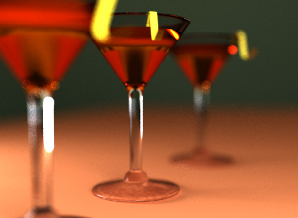
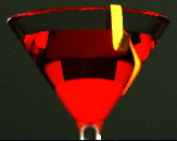
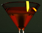
Rendered scene
As it turned out, the final rendered scene made comparatively little (but noticeable) use of the major techniques implemented, i.e. photon mapping for caustics, volume rendering, and Fresnel glass. It would have been nice to have chosen a scene which more aggressively demonstrated those techniques. Also, I found the lighting of the original photograph very difficult to simulate, even with a real martini glass. Even with many tries, I was unable to obtain the correct lighting conditions in the rendered scene that gave the nice specular highlights off the base of the glass as seen in the photograph. Nevertheless, it was nice to see the yellowish reflection of the left window in the red liquid (upper-right corner of the middle glass) which was also present in the original photograph but at a different location. Also, the size of the "cone" of darkness in the middle of the liquid agrees with that of the photograph, i.e. a larger cone for the glass that is further away - this came out naturally as a consequence of the modeling.
The final image made use of 2025 samples per pixel (!) to achieve low noise and good depth of field effect, with 300,000 caustic photons and 100,000 volumetric photons. The radiance estimate was computed using 100 photons. A lot of the caustic photons were not productive because they hit other areas of the glasses; it would have been more productive to concentrate the photons on the base of the glasses where they have the most effect.
Source code
The source code can be found here.