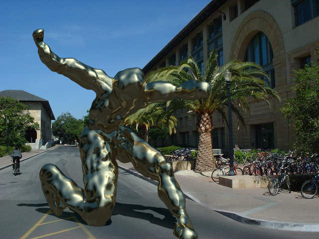
My final project was to place a synthetic sculpture in a real scene. I had originally planned to actually replace the fountain outside of the Gates building with something else, but I ran out of time and so just put one nearby (though you might notice that the fountian is indeed missing from reflections).
This project entailed several issues. The first was just creating the sculpture itself; I hadn't seen any readily available tool such as Maya which had the flexibility and ease-of-use required for sculpting on the computer. Once I created the sculptures I of course had to figure out an efficient way to ray-trace them. To get realistic lighting I had to construct an environment map of the area outside Gates, and again, had to to incorporate this into the ray-tracer. To get a more realistic surface detail on the sculpture I decided to work on a variation of hypertexture - while my original plan was to simulate chisel marks, porous stone, etc. it turned out I didn't have time to do that, but what I did implement was useful in directly simulating microfacets for a glossy, rough aluminum look. Finally, the synthetic image had to be composited with a real photo, taking into account shadows.
For their extreme flexibility, simplicity, and ability to produce complex smooth surfaces I chose to represent sculpted surfaces with levelsets (of signed distance functions sampled on regular cartesian grids). However, a levelset of size O(n^3) only shows a surface of O(n^2) complexity; clearly they would not scale to the resolution I wanted (250^3 grids or higher), both in terms of storage and computation. This problem has been solved by others using octrees instead of grids. However, for real-time work I suspected that all the overhead involved with octrees would not be worth their asymptotic scalability. Instead I used a simpler two-grid approach, storing a coarse grid of side length O(n^0.75) filled with pointers to fine subgrids (each of side length O(n^0.25)) where the surface intersects the coarse voxels. The coarse grid also had inside/outside flags to help in sculpting operations. This data structure scales like O(n^2.25) in storage and cost, but with small constants which made it ideal for the regime I was interested in, namely n=30 up to n=1000 or so.
My sculpting tool renders the levelset in OpenGL efficiently by exploiting the coarse grid. The algorithm sweeps through the coarse grid, performing frustum culling and level-of-detail analysis. Coarse voxels which appear small enough on screen are splatted as single points (with a normal taken from the gradient of the function in the fine subgrid); larger voxels have their fine subvoxels splatted similarly; even larger voxels use a simple marching-cubes-like approach to quickly triangulate the surface; and the largest voxels use the same triangulation but with nodes moved to the surface and smooth vertex normals.
I provide two tools, a push/pull operator and a smooth/roughen operator. Whenever the user clicks or drags, a ray is traced from the camera through the mouse pointer to the levelset, and the levelset is locally evolved with motion in the normal direction or motion by mean curvature respectively. The evolution is weighted by distance from the surface point, up to some maximum radius controlled by the user. (The speed of evolution is similarly controlled). During these operations, it is important to keep the function signed distance, which I achieve using the fast sweeping method locally. It is also necessary to keep track of when the surface moves to an unpopulated coarse voxel or completely leaves a populated coarse voxel, and update accordingly.
The user begins sculpting on a 30^3 grid, but can refine (using tricubic B-spline subdivision) to 60^3, 120^3, 240^3, etc.
The two-grid structure also makes for efficient ray-tracing. After clipping to the bounding cube, I march through the coarse grid with a DDA algorithm. Whenever I hit a populated coarse voxel, I trace through the fine subgrid, taking steps of size equal to the distance from the boundary (which is what the levelset function gives me). I evaluate the levelset function using trilinear interpolation for speed while I've far away, but then switch to a C2 tricubic Hermite interpolation near the surface for good smoothness. (To construct this C2 surface I begin with the C1 Catmull-Rom interpolation, then perform symmetric Gauss-Seidel iterations on the first derivatives to quickly get to C2). If I detect I'm at a grazing angle (where the steps are too small since the ray is close to the surface) I steadily grow the stepsize to avoid slowdown. Finally, once I detect a sign change (going from inside to outside or vice versa) I use the secant method to solve for the zero level. I use the exact, analytic derivative of the function to compute a normal.
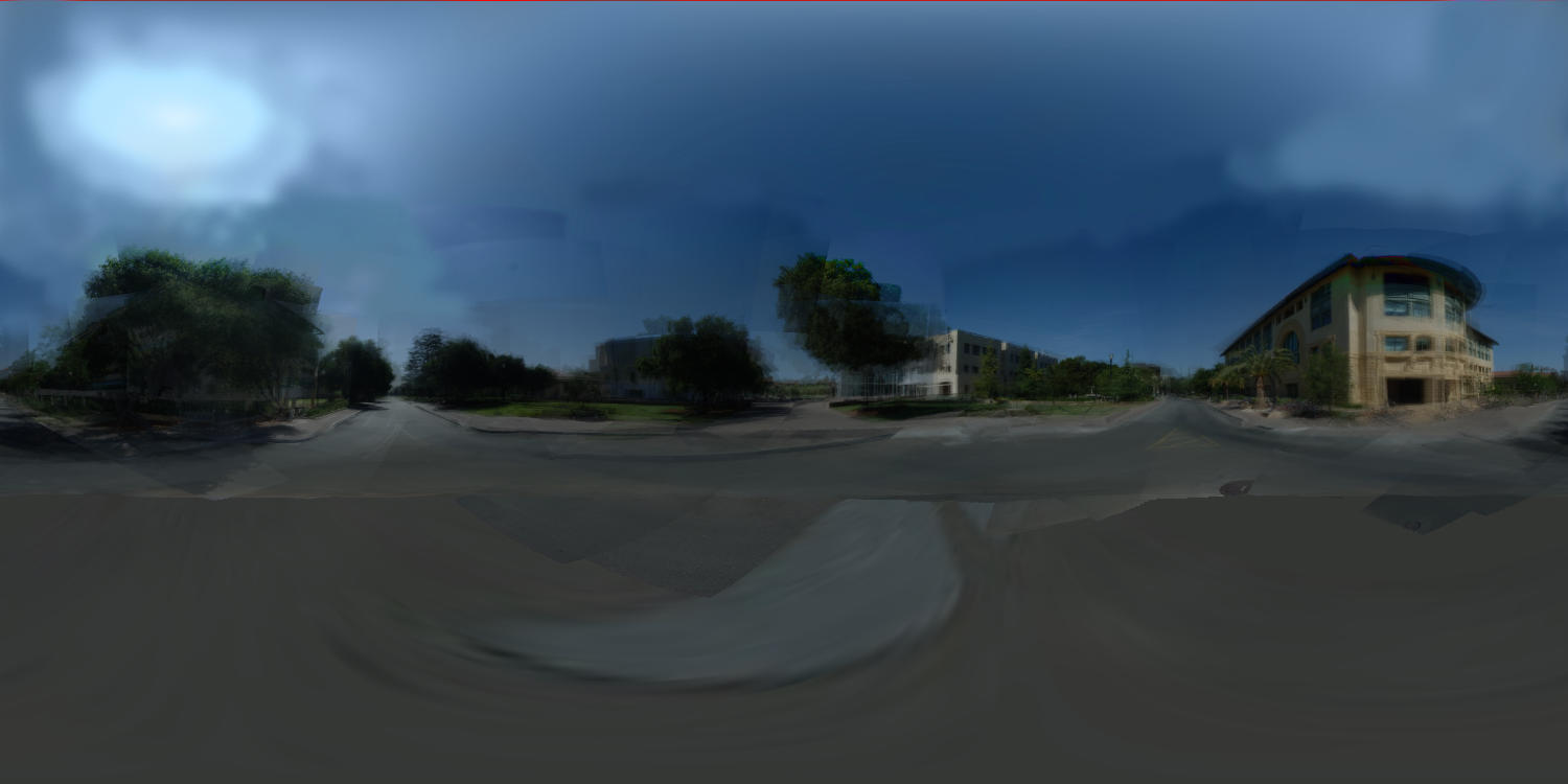
I originally has hoped to replace the fountain, so I needed to do something more tricky than just photographing a silvered ball for the environment map. Instead, I took 70+ digital photos of the area around the fountain, and stitched them together avoiding the fountain altogether.
Since the photos were uncalibrated - position, orientation, exposure, etc. of my camera were all unknown - I had to do some kind of a structure solve to recover the camera poses. Luckily the focal length etc. was constant (I measured it to be a 22.5 degree field of view with a 4x3 aspect ratio). I also measured the size of the fountain (it's essentially 4 metres across diagonally). Then by hand I identified a number of points common to multiple photos, such as the top of a signpost or a corner of a building. Then using the known locations of the corners of the fountain I solved (using MATLAB) for the poses of the cameras that could see the fountain, then from these figured out a least-squares solution for the 3d positions of other points those cameras could see, and continued to iterate back and forther between known points and known cameras.
Once I had the poses, I assembled a very simplified geometrical representation of the scene (essentially a 10 sided prism). I first projected CIE standard clear-sky model onto this scene, then one by one projected and blended in the photographs (after rescaling them to try to match their exposure, and masking out bad pixels from the fountain or passers-by). Finally, I used photoshop to smooth other boundaries between photos and fill in a few holes.
To improve surface detail I had the idea of adding a small-length-scale random perturbation to my levelset function, which would perturb the surface with it. This is essentially a simplified form of hypertexture, using signed distance instead of density, and addition instead of various min/max/etc operations. This perturbation function would be periodic (i.e. only a single tile would be stored). It could be constructed to simulate things such as chisel marks, concrete or conglomerates, porous stone, etc. It could be easily incorporated into the ray-tracer, simply by adding to the evaluation, which was already pretty robust with the secant solver, just making sure that the perturbation had gradient less than 1). Unfortunately I only had time to implement trilinear interpolation and a slightly smoothed random texture, which is not good enough for visible texturing.
Example: hand without texture, hand with too much rough texture: 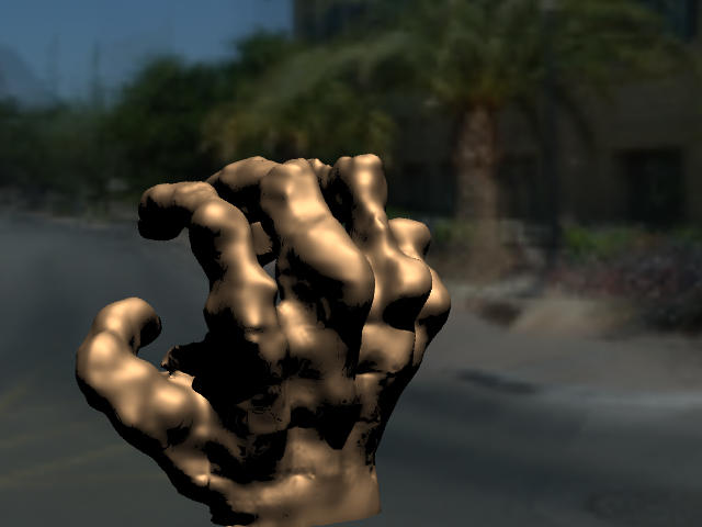
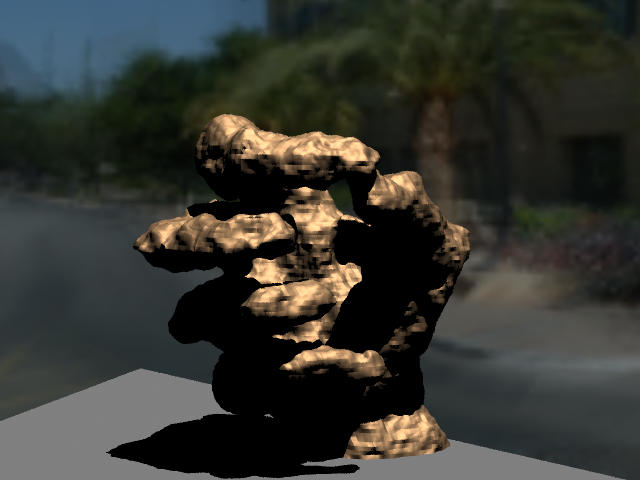
I also didn't have time to experiment with global illumination and more advanced BRDF's. However, after seeing Kurt Akeley's presentation at the contest, I realized my existing implementation was perfect for directly simulating microfacet models with just the Whitted algorithm. I simply needed to reduce the length-scale of the perturbations to below pixel size, at which point the texture really became just a microfacet distribution. For the Monte Carlo simulation I sent in about a 100 rays per pixel, with the surface material just a mirror ("shinymetal").
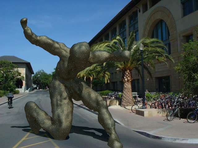
Examples of the final image with no microtexture and with more microtexture.
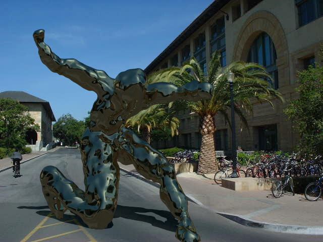

Finally, there was the issue of compositing the synthetic images with the real photos. I wanted shadows from the sculpture to fall onto the ground in the photo, so I used Debevec's differential rendering idea. I augmented lrt with flags that could make object invisible to rays coming directly from the eye, but visible on all subsequent bounces. Then I could render just the ground plane, then the ground plane with shadows from the object (and using a distant point light source where the sun was, computed again from CIE formulas in the IES handbook) but no object visible above it. The difference of the two images gave the shadows. I could add the shadows to the original photo (scaled down to account for indirect illumination). Finally, the sculpture rendered without ground plane can be composited "atop" of that. The illumination map is of course not directly visible.
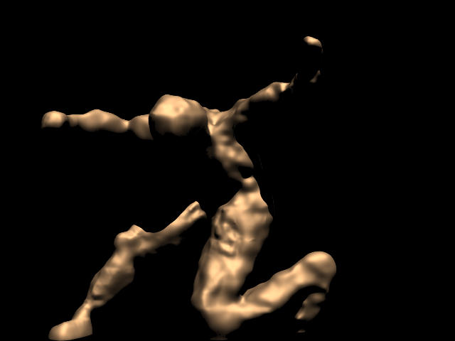
The various source images for a composited image (with just a plastic
material for the figure, no microfacets): 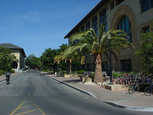


I put everything in one big .tar.gz, but organizated into subdirectories. Unfortunately I didn't save some of the throw-away MATLAB scripts to export the solved camera poses, but I'm including those output files so nothing is lost.